Loan Default Prediction
This website showcases our final project for FIN 377 - Data Science for Finance course at Lehigh University.
Table of contents
Introduction / Proposal
The big question that we are trying to answer in our project is “How effectively can we use macroeconomic in conjunction with ordinary risk factors to effectively predict loan defaults?”. Specifically, we will look at problems such as:
- How do macroeconomic factors such as unemployment rates, that vary based on geography, relate to and effectively predict loan defaults within that region?
- How do broad market conditions, such as inflation and changes in inflation, relate to and help predict loan defaults?
- How do individual loan metrics such as LTV, interest rate, loan term, and loan amount relate to and predict loan defaults?
- How does an individuals income, compared to the state median/mean gross income, relate to and predict loan deafults?
- Our project will compare the performance of a baseline model that uses the variables in the base dataset to predict loan defaults with a model that uses additional macroeconomic variables discussed above. We will evaluate how well adding this external data to the model improves the variables, and carryout additional analysis on how these external variables affect the results (which help the least/most).
Methodology
We outlined and completed this project through steps of:
- Data Collection
- EDA
- Pre-processing
- Base Model
- Initial Macro Model
- Interaction Macro Model
Data Collection
lending = pd.read_csv("input/lending_data.csv")

inf = pdr.DataReader(["T5YIE"], "fred",datetime(2005,1,1), end =datetime(2022,4,1) )
inf.to_csv("input/inflation_exp.csv")

stfips = pd.read_csv("dev/state_fips.csv",skipinitialspace=True)

state_list = pd.DataFrame(lending["addr_state"].unique())
state_list = stfips.merge(state_list, on = "state", how  = "left")
We read lending data that we downloaded from kaggle. This is our main dataset and what we build off of to incorporate other variables for our algorithm. Additionally included is some of the add-on data and modifications such as inflation from FRED.
You can see the full download_data notebook here.
EDA - Exploratory Data Analysis
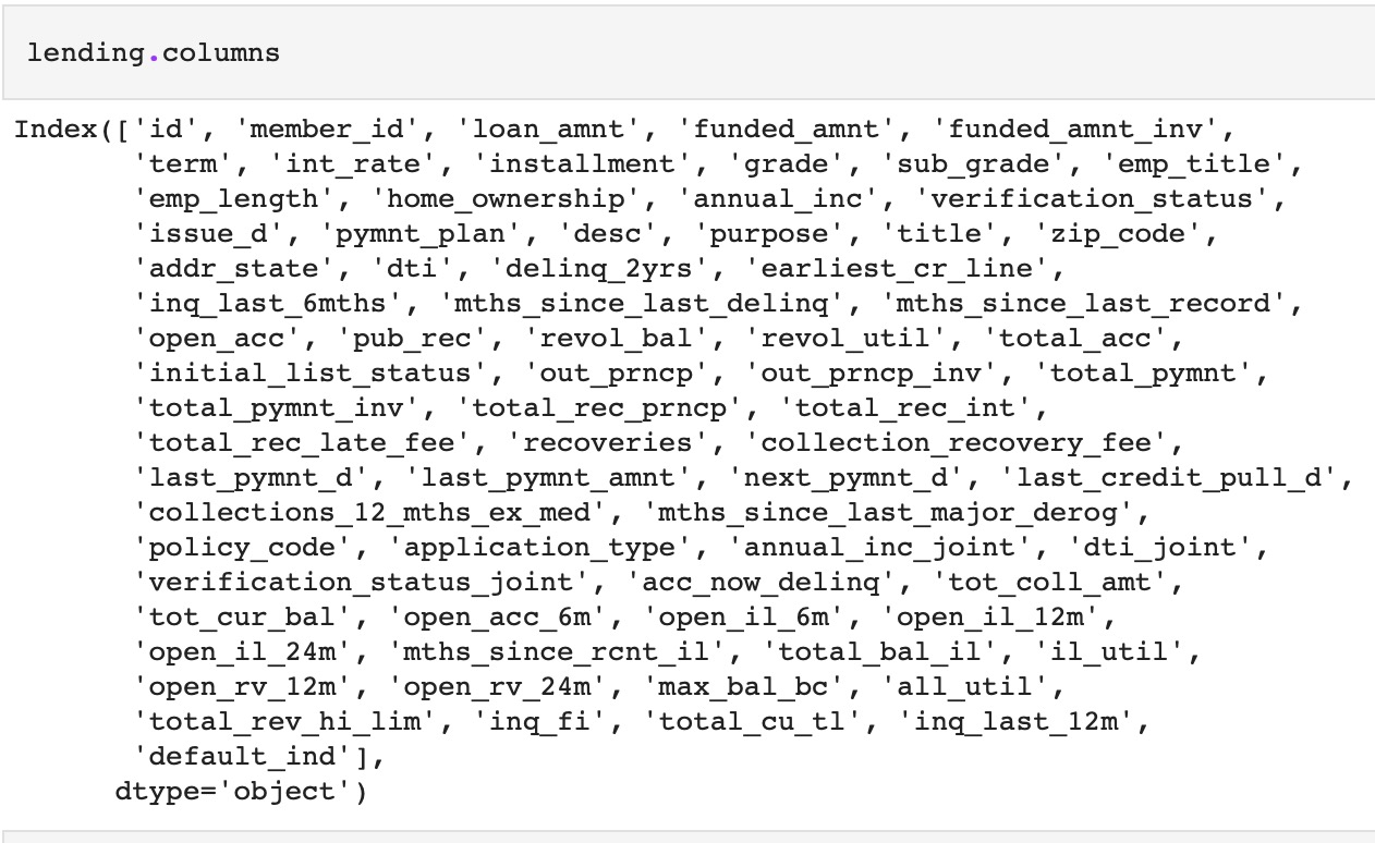
print('There are',lending.shape[1],"columns")
lending.columns

lending.describe().T.style.format('{:,.2f}')

lending.describe(percentiles=[.01,.05,.95,.99]).T.style.format('{:,.2f}')

(
    (lending.isna().sum(axis=0)/len(lending)*100)
    .sort_values(ascending=False)[:13].to_frame(name='% missing') .style.format("{:.1f}")

    perc = 84.0
    min_count =  int(((100-perc)/100)*lending.shape[0] + 1)
    lending = lending.dropna(axis=1,thresh=min_count)
)
EDA is crucial to prepare data for machine learning. Above are main examples of EDA we did mostly on our base dataset, lending. We do this to better understand the data we are dealing with and how to best utilize it. The code shows us the columns, data shape, variabable summary statistics, percentiles, and even variables with missing values and what percentage is missing. We also dropped variables that had over 84% of values missing, as seen in the last code block.
Below are some examples of Visual EDA that we did to get a better sense of how variables relate to each other and observe major trends.
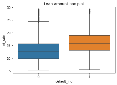
Loans that are defaulted have a higher interest rate, generally.
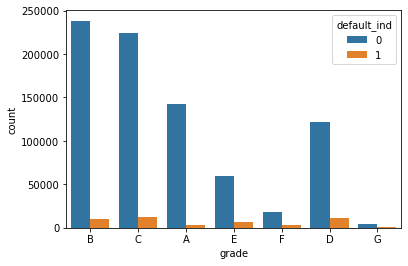
Doesn’t seem to be any noticeable trends in loan grade and defaults.
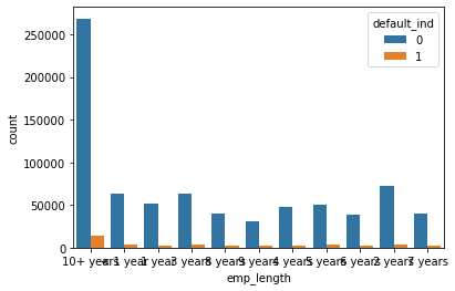
Longer loans by far have more defaults but also by far more loans.
You can see the full status_report notebook of EDA here.
Pre-processing
lend = lending.drop(['default_ind' ], axis = 1)
rng = np.random.RandomState(0)

X_train, X_test, y_train, y_test = train_test_split(lend, y, stratify = y, test_size = 0.2, random_state = rng)

num_pipe = make_pipeline(SimpleImputer(), StandardScaler())
cat_pipe = make_pipeline(OneHotEncoder(handle_unknown='ignore'))

num_pipe_features = X_train.select_dtypes(include = "number").columns
num_pipe_features = [e for e in num_pipe_features if e not in dont_use]

preproc_pipe = ColumnTransformer(
    transformers = [
    ('num', num_pipe, num_pipe_features),
    ('cat', cat_pipe, cats)],
    remainder = 'drop'
)
Exemplified is our pre-model adjustments and setup. We dropped default indicator of course to avoid data leakage, and created random state. We split our data into testing and training data at a 80/20 split and stratified y to ensure the best representation of data. We created the number pipe using SimpleImputer and StandardScaler as usual, and the categorical pipe using OneHotEncoder. We selected numerical variables from the training data to be processed through the number pipe and vice versa, making sure to not use certain variables that we ruled out of our model.
Thus, we created our preprocessing pipe by using ColumnTransformer, combining the numerical pipe & features as well as the caategorical pipe & features, dropping the rest.
Base Model
logit = make_pipeline(preproc_pipe, LogisticRegression(max_iter = 1000))
logit.fit(X_train, y_train)
y_pred = logit.predict(X_test,)
print(classification_report(y_test, y_pred))
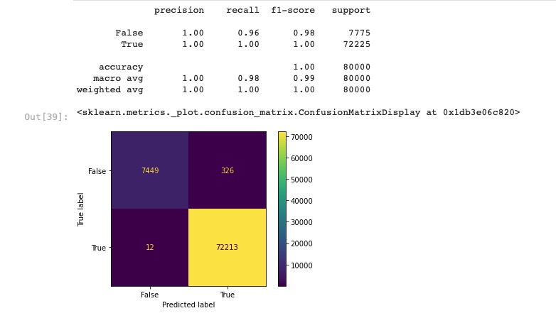
ConfusionMatrixDisplay.from_estimator(logit, X_test, y_test)
We created a logit model using the preprocessing pipeline, fit it to the training data, and predicted y test with our base model. We outputted the classification report and the confusion matrix for the model which can be seen below.
Next:
def custom_prof_score(y, y_pred, roa=0.02, haircut=0.20):
    """
    Firm profit is this times the average loan size. We can
    ignore that term for the purposes of maximization.
    """
    TN = sum((y_pred == 0) & (y == 0))  # count loans made and actually paid back
    FN = sum((y_pred == 0) & (y == 1))  # count loans made and actually defaulting
    return TN * roa - FN * haircut
# so that we can use the fcn in sklearn, "make a scorer" out of that function

prof_score = make_scorer(custom_prof_score)
We defined a profit function that we wanted to focus on as we are maximizing profit for a lending company.
Then:
pipe = Pipeline([('columntransformer',preproc_pipe),
                 ('feature_create','passthrough'),
                 ('feature_select','passthrough'),
                 ('clf', LogisticRegression(class_weight='balanced', max_iter = 1000))
                ])

param_grid = [

    # baseline: last class's 3 variable logit, no feature creation or selection
    {'columntransformer': [preproc_pipe]},

    # now, try different feature selection methods (no creation, logit as estimator)
    dict(feature_select=['passthrough',
                          SelectKBest(f_classif,k=10),
                          SelectKBest(f_classif,k=20),
                          SelectKBest(f_classif,k=30),
                          ]),

    # now, try different feature creation methods (and possibly reduce the features after)
    {'feature_create': [
                        # this creates interactions between all variables
                        'passthrough'],
     'feature_select': ['passthrough']
    },

]

grid_search = GridSearchCV(estimator = pipe,
                           param_grid = param_grid,
                           cv = 5,
                           scoring=prof_score
                           )

results = grid_search.fit(X_train,y_train)
We created a pipeline to grid search with, and defined paramters. We used feature selection with “Kbest” and conducted a grid search using default CV of 5. We fit on the train data and outputted best estimator results which showed that no feature selection yielded the highest mean test score.
You can see the full Base_Data_model here.
Initial Macro Model
lending = pd.read_csv("dev/lending_merge.csv")
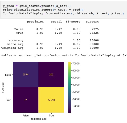
This is truly the main difference between the macro model and the base model. Everything else was conducted and measured in the same way (pipelines, parameters, grid search, etc) and resulted in a lower mean test score than the base model with the same, best model of passthrough of feature selection and creation.

The macro-merged data was created using some of the following code:
lending = pd.read_csv("input/lending_data.csv")
inflation_exp = pd.read_csv('input/inflation_exp.csv')
state_fips = pd.read_csv('dev/state_fips.csv')
med_inc = pd.read_csv('dev/med_inc.csv')
mean_inc = pd.read_csv('dev/mean_inc.csv')
state_unemp = pd.read_csv('dev/state_unemp.csv')
Read in all of the data we want to combine
lending['issue_d'] = pd.to_datetime(lending['issue_d'])
lending_h = lending
med_inc['DATE'] = pd.to_datetime(med_inc['DATE'])
mean_inc['DATE'] = pd.to_datetime(mean_inc['DATE'])
state_unemp['DATE'] = pd.to_datetime(state_unemp['DATE'])
inflation_exp['DATE'] = pd.to_datetime(inflation_exp['DATE'])

med_inc['year'] = med_inc['DATE'].dt.isocalendar().year
mean_inc['year'] = mean_inc['DATE'].dt.isocalendar().year
state_unemp['year'] = state_unemp['DATE'].dt.isocalendar().year
inflation_exp['year'] = inflation_exp['DATE'].dt.isocalendar().year
Convert data so to have common types.
lending_x["mean_inc"] = 0
for i in range(400000, len(lending_x)):
    for state in mean_inc.columns[1:-1]:
        if state == lending_x["addr_state"][i]:
            for year in mean_inc["year"]:
                if year == lending_x["year"][i]:
                    df = pd.DataFrame(mean_inc.loc[state_unemp['year'] == year])
                    lending_x["mean_inc"][i] = df[state]
Agorithm used to index match annual data from the macro datasets and add it to the client dataset.
state_list = stfips.merge(state_list, on = "state", how  = "left")
state_list["statecode"] = state_list["state"].astype(str)+state_list["code"].astype(str)

inflation_yr = inflation_exp.groupby(['year']) ['T5YIE'].mean().to_frame()
inflation_yr = inflation_yr.reset_index()

lending_merge = lending_h.merge(inflation_yr, how = "left", on = 'year')
Finalize data and combine.
You can see the full Macro_Data_model here.
Interaction Macro Model
mean_mean_inc = lending["mean_inc"].mean()
mean_med_inc = lending["med_inc"].mean()
for i in range(0,len(lending)):
    if lending["mean_inc"][i]==0:
        lending["mean_inc"][i] = mean_mean_inc
    if lending["med_inc"][i]==0:
        lending["med_inc"][i] = mean_med_inc

lending["skew"] = (lending["mean_inc"]/lending["med_inc"]).round(2)
lending["inc/mean"]= (lending["annual_inc"]/lending["mean_inc"]).round(2)
lending["inc/client_mean"]=(lending["annual_inc"]/lending["annual_inc"].mean()).round(2)
lending["inc/client_med"]=(lending["annual_inc"]/lending["annual_inc"].median()).round(2)
lending["int-inf"] = lending["int_rate"]-lending["T5YIE"]
lending.head(5)
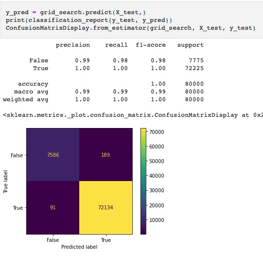
The model was conducted and asssessed the same way as prior models (pipelines, parameters, grid search, etc) however we created these interactions into the data at the very beginning because we felt that the macro data was not being fully utilized as it wasn’t related to specific clients. This was our attempted solution and it resulted in a slightly higher mean test score in teh same model type.

You can see the full Macro2_Model here.
Analysis
We attempted to best predict loan defaults using not only consumer lending data but also macro-economic variables/factors. In that we created our three models, only to arrive at our base data model doing the best. However, our progress by adjusting the macro model to include interaction variables gives us hope and further inspiration of what we could create. In hindsight, of course the macro variables aren’t going to be useful on their own as they don’t tie to specific loans. We realized this and attempted to incorprate them into each loan to help the algorithm better predict defaults. With more time, perhaps different model types, and a better understanding of machine learning we are confident we could continue to develop the merged macro data into a strong machine learning algorithm.
Resulting Test Matrices
The base model is the most “aggressive” model in that it predicts the least amount of defaults, opening the door for the most profit. Having just the client data, it doesn’t have broader market factors to be weary of in its predictions.
The initial macro model is more “conservative”, and the least profitable. We did not manipulate any of the macro variables other than standard imputing/dropping. The model seems to be very timid to market conditions resulting in an over-prediction of loan defaults. As a result, it correctly predicts more clients that would actually default.
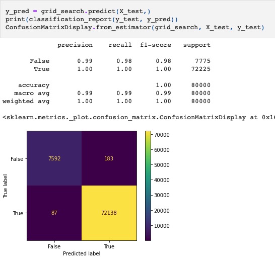
Finally, the interaction macro model is the most “conservative”. Despite being most conservative, it is not the least profitable. Of course, this is entirely dependent on the assumptions made in your profitability scoring. This model predicts the most loan defaults and subsequently the most correct actual loan defaults.
About the Team

Wasti is a Senior ‘22 Finance major with minors in Data Science and Mathematics. Upon graduation he will return to Lehigh as a Masters of Financial Engineering candidate.

Eric is a Senior ‘22 Finance major. Upon graduation he will begin his career as a Financial Services Advisory Associate at KPMG in their NYC Office.

Colin is a Senior ‘22 Finance major with a minor in Psychology.
More
To view the GitHub repo for this website, click here.